Phi is the 21st letter in the Greek alphabet with a value approximately equal to 1.618. As we shall see, Phi is also a magical number, better known by its popular moniker, the “Golden Ratio” or the “Golden Mean”.
Part of the allure of the Golden Mean is that it shows up in many natural forms. Perhaps the most familiar example is the spiral shape of the nautilus shell, which has an uncanny resemblance to the spiral generated by a logarithm function proportional to the Golden Mean.
For millennia, the Golden Mean has also mesmerized artists and designers who utilized it to create visually pleasing shapes. Leonardo Da Vinci used the Golden Mean to compose “The Last Supper.” Le Corbusier and Salvador Dali are said to have proportioned their works to approximate the Golden Mean, particularly in the form of the Golden Rectangle, believing this proportion to be aesthetically pleasing.
My intention is not to give a detailed history of this magical number, nor to provide an exhaustive list of where the Golden Mean manifest in nature, art and science. My goal is to show a lesser known fact: that the orderly structure implied by the Golden Mean is consistent with a random process. This surprising result was proved in 1986 by three mathematicians: R. Dan Mauldin, S. Gray and S. Williams (MGW) [1]. It is surprising because the path of random processes are disorderly. Yet, MGW’s theorem shows that there can be subtle order in the “chaos”. The unexpected connection between two vastly different realm of nature also makes their discovery a beautiful one. I will now summarize the gist of this discovery, omitting most of the technical details.
Let’s begin with a picture to visualize the appearance of Phi. What better example to use than the nautilus spiral? Figure 1 (a) shows a rectangle with sides of length A and B where A < B. Let r denote the ratio A/B. Divide this rectangle into a square of side A and a new rectangle. If the ratio of the lengths of the sides of this new rectangle, (B-A)/A also equals r, then both the original rectangle and the new one are “Golden Rectangles”, and r is the Golden Mean (let’s call it M from now). The value of M is 1.61803399, which is the value of Phi. Importantly, M can be obtained as 

We can of course continue the process of dividing a golden rectangle indefinitely. If we do so, we get a Nautilus-like spiral. We identify this spiral mathematically as the logarithm spiral. Defined in polar coordinates by 

The Golden Mean shows up in many other places. The way tree branches form or split is an example of the Fibonacci sequence (0, 1, 1, 2, 3, 5, 8, 13, 21, 34 …). This sequence relates directly with the Golden Mean since if you take any two successive Fibonacci numbers, their ratio is very close to the Golden Mean. Moreover, as the numbers get higher, M becomes even closer to 1.618 (example: the ratio of 3 to 5 is 1.666, but the ratio of 13 to 21 is 1.625 and so on).

The Golden Spiral is also found in root systems, pine cones, the petals of flowers like the Sunflower, patterns on snails and seashells, hurricanes, the spirals of galaxies and even the DNA molecule, which measures 34 angstroms by 21 angstroms at each full cycle of the double helix spiral, and 34 and 21 are consecutive numbers of the Fibonacci sequence [2].

Given the ubiquity of the Golden Mean, you may ask: is there more to the Golden Mean that meets the eye? In particular, is it the child of some fundamental mathematical principles? The answer is yes, according to Mauldin, Graf and Williams.
The gist of MGW’s theorem is the following number experiment [3]. Choose a number x randomly from a uniform distribution on the interval [0,1]. Then between x and 1, choose y at random from the uniform distribution on [x,1]. Hence, we have two intervals ![J_1 = [0,x]](https://s0.wp.com/latex.php?latex=J_1+%3D+%5B0%2Cx%5D+&bg=ffffff&fg=3a3a3a&s=0&c=20201002)
![J_2 = [y,1]](https://s0.wp.com/latex.php?latex=J_2+%3D+%5By%2C1%5D+&bg=ffffff&fg=3a3a3a&s=0&c=20201002)


The result is a Cantor set, where its Hausdorff dimension 


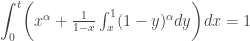
Applying some calculus shows that

That the Golden Mean should emerge as the dimension of randomly constructed numbers (Cantor sets) is counter-intuitive. It raises all sorts of philosophical questions concerning “the nature of nature” and the role of chance and God in creation. These are interesting and profound questions which I leave you to ponder.
Glossary
Hausdorff dimension
The Hausdorff dimension generalizes the notion of dimension to irregular sets such as fractals. For instance, a Cantor set has a Hausdorff dimension of ln2/ln3, the ratio of the logarithm to the base 2 of the parts remaining to the whole after each iteration.
Cantor Set and Random Cantor Set
The classical triadic Cantor set (named after George Cantor) is obtained by dividing the unit line into three equal parts, discarding the middle part, keeping the remaining parts, then repeating the operation with the two remaining parts ad infinitum. In the random version, it could be any of the three parts that is discarded at random after each division.
Notes:
[1] R. Daniel Mauldin, S. Grafand S. Williams (1986), “Random Homeomorphisms”, Advances in Mathematics, 60(1986), 239-359.
[2] For more fascinating research on the Golden Mean structure of DNA, see http://creationwiki.org/Jean-claude_Perez#cite_note-4
[3] This section is a lightly edited version of R. Daniel Mauldin (1987,)”Probability and Nonlinear Systems,” Los Alamos Science, No. 15, Fall , 52-90. Reprinted in N.C. Cooper (ed.), From Cardinals to Chaos, Cambridge University Press, 1989.